|
Size: 8560
Comment:
|
Size: 8698
Comment:
|
| Deletions are marked like this. | Additions are marked like this. |
| Line 4: | Line 4: |
| ''This is a holding page to gather together notes on producing an analytic vignetting model for eSASS tasks'' | ''Please not that this information is out of date and does not represent the vignetting function in the eSASS users release from 200602.'' This is a holding page to gather together notes on producing an analytic vignetting model for eSASS tasks |
Modelling the vignetting function of eROSITA
Please not that this information is out of date and does not represent the vignetting function in the eSASS users release from 200602.
This is a holding page to gather together notes on producing an analytic vignetting model for eSASS tasks
Problem: The current method to represent the eROSITA vignetting function in the eSASS required interpolation from a tabulated grid of calibration measurements, this is computationally awkward, and can lead to discontinuities in the derived system response.
Desired improvement: Compute an analytic description of the vignetting function of each eROSITA telescope module, and save the parameters of this model into the CALDB.
Zeroth order model (TD)
Input data
- Start from the vignetting description file supplied with the current version of SIXTE
i.e. the file share/sixte/instruments/srg/erosita_vignetting_v2.1.fits supplied in the SIXTE instrument description package v1.4.0
- The file contains a list of vignetting values evaluated for broad energy bands and for many offaxis angles
- The vignetting is tabulated over 3 energy ranges: 0.0-2.5, 2.5-5.5 and 5.5-20 keV (in comparison eSASS uses energy ranges: 0.0-2.5, 2.5-5.5 and 5.5-10 keV)
- it is not clear what average or effective energy should be assumed for each energy band, for simplicity we assume 1.25keV, 4.0keV and 7.5keV.
- The vignetting is tabulated at 31 off-axis angles (from 0.0-30arcmin) for each energy band
- A single description is used for the vignetting functions of all eROSITA FMs/TMs
Derivation of model parameters
See the gnuplot script used to do this: derive_analytic_vignetting_coeffs.plot
- For each energy value we fit a simple model to the vignetting as a function of off-axis angle (θ)
- For illustrative purposes we assume a uniform 1 sigma uncertainty of 1e-3 per data point
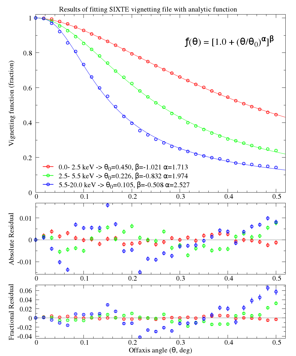
After some trial and error, a distribution of the form: vign(θ) = [1.0 + (θ/θ0)α]β was found to give a reasonable match to the tabulated values
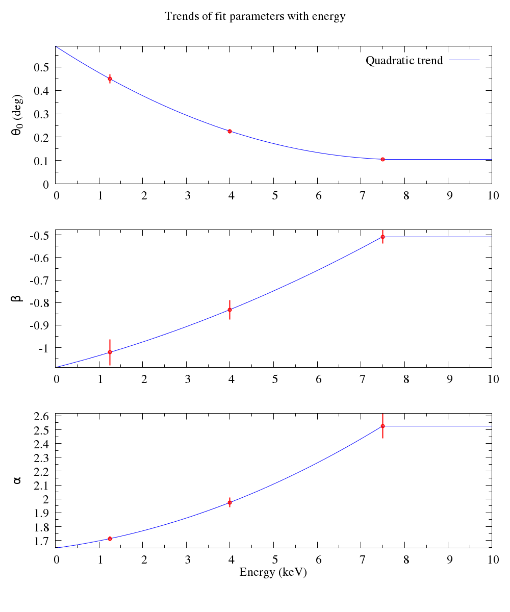
The values of the θ0,β,α parameters are then interpolated using a quadratic expression to allow evaluation of the expression at any energy
- This quadratic form does strange things at energies above the upper tabulated energy band and so the vignetting model is assumed to be constant in energy above 7.5keV
- future versions will be based on more energy bands (five or six?) than the three available here
Figures demonstrating the fit


The parameters describing the model
Results of fits at each energy:
- functional form is:
vign(θ,θ0,β,α) = [1.0 + (θ/θ0)α]β
- where
- θ = off-axis angle in degrees
θ0 is a scaling parameter, also in degrees
- α, β are dimensionless exponents
- independent fits at each of [1.25, 4.0, 7.5] keV give:
Energy=    1.25 keV: theta0= 0.44966 +-  0.02004  beta=-1.02111 +-  0.05693  alpha= 1.71288 +-  0.01767
Energy=       4 keV: theta0= 0.22575 +-  0.00860  beta=-0.83151 +-  0.04289  alpha= 1.97408 +-  0.03523
Energy=     7.5 keV: theta0= 0.10547 +-  0.00350  beta=-0.50753 +-  0.03063  alpha= 2.52732 +-  0.09069
we can describe this as a matrix of coefficients [3 coeffs X Nenergies]
coeff[1,1],coeff[2,1],coeff[3,1] = [ 0.44966, -1.02111, 1.71288]
coeff[1,2],coeff[2,2],coeff[3,2] = [ 0.22575, -0.83151, 1.97408]
coeff[1,3],coeff[2,3],coeff[3,3] = [ 0.10547, -0.50753, 2.52732]
Since we only have three data points in energy, we use Lagrangian polynomial interpolation (https://en.wikipedia.org/wiki/Lagrange_polynomial)
- i.e if we have three points on the plane at (x1,y1), (x2,y2), (x3,y3), the quadratic equation that passes through all of them is given by:
lagr(x,x1,x2,x3,y1,y2,y3) = y1*((x-x2)/(x1-x2))*((x-x3)/(x1-x3)) + y2*((x-x1)/(x2-x1))*((x-x3)/(x2-x3)) + y3*((x-x1)/(x3-x1))*((x-x2)/(x3-x2))
- Therefore, energy dependent versions of theta0,beta,alpha are given by
f_theta0(energy) = lagr(clip(energy),e[1],e[2],e[3],coeff[1,1],coeff[1,2],coeff[1,3])
f_beta(energy)   = lagr(clip(energy),e[1],e[2],e[3],coeff[2,1],coeff[2,2],coeff[2,3])
f_alpha(energy)  = lagr(clip(energy),e[1],e[2],e[3],coeff[3,1],coeff[3,2],coeff[3,3])
- It is necessary to limit the extrapolation at high energies:
emin = 0.0
emax = 7.5
clip(eraw) = (eraw<emin?emin:(eraw>emax?emax:eraw))
- And so the general vignetting function is:
vign_gen(oa,energy) = vign(oa,f_theta0(energy),f_beta(energy),f_alpha(energy))
In the future we will have more energy intervals to consider and so a more sophisticated method will be needed to fit the trends of θ0,β,α as a function of energy
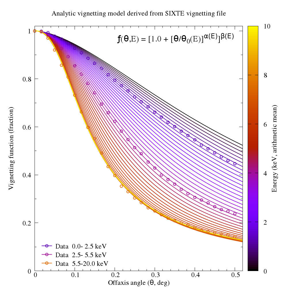
- The resultant analytic vignetting model is illustrated in the figure below:

Description of model in CALDB
- See script: "/home/erosita/sw/eSASSdevel/erosita/task/srctool/scripts/build_avign_caldb_files.csh"
example CALDB file: tm1_avignet_010101v01.fits
- File format:
- One row per energy band
- Columns: Name, FITS format, [unit]
- ENERGY DE [keV]
- COEFFS 3D [degree,-,-]
- OA_X 1D [pix]
- OA_Y 1D [pix]
- PIXSCALE_X 1D [deg/pix]
- PIXSCALE_Y 1D [deg/pix]
- Note that thhe columns OA_X,OA_y,PIXSCALE_X and PIXSCALE_Y allow for a very general case where the pixel scale and the coordinates of the optical axis are assumed to be energy dependent
Using the analytic vignetting model in eSASS
- See module eSASS "/home/erosita/sw/eSASSdevel/erosita/task/srctool/srctool_generic_avign_mod.f90"
- The Analytic vignetting model described above is implemented in SRCTOOL versions v1.17 and later
- Instructions of how to use the module are given below:
  !--------------------------------------------------------------------------------
  !
  !  HOW TO USE THESE ROUTINES
  !  =========================
  !
  ! 1) Include this module in the calling module:
  !
  !  use srctool_generic_avign     ! use generic analytic vignetting model routines
  !
  !  And make sure that this file is listed in the Makefile modules variable for your task
  !
  ! 2) At the beginning of the calling routine define an avign data type (one for each instrument):
  !
  !    type(avign_type)   :: avign             ! an avign for a single instrument
  !
  !    alternatively:
  !
  !    type(avign_type), dimension(7) :: avign_list  ! array of avigns for all instruments
  !
  ! 3) Always initialise the avign data structure before use:
  !
  !    call avign_empty_avign(avign)
  !
  ! 4) Read the avign coefficients from the CALDB for each instrument (giving the instrument name,
  !    and the observation start+end date strings) and check the value of the resulting ierr status flag
  !
  !    call avign_read_avign_from_caldb(avign, instname, date_obs, date_end, ierr)
  !
  !    if ( ierr .ne. 0 ) then
  !      call wrerr (subroutinename, ierr, "Problem reading AVIGN from CALDB")
  !      return
  !    end if
  !
  ! 5) [Optional] Report the contents of the AVIGN calibration file to stdout
  !
  !    call avign_report_avign_info(avign)
  !
  ! 6) Call the relevant routine to compute the value of the vignetting function for a given
  !    pixel position (raw coordinate system) and photon energy (keV):
  !
  !    call avign_calc_vign_at_xye(avign, x, y, energy, vign, ierr)
  !
  ! 7) Repeat step 6) as many times as required
  !
  ! 8) when finished, free up the allocated memory
  !
  !    call avign_empty_avign(avign)
  !
  !-------------------------------------------------------------------------------
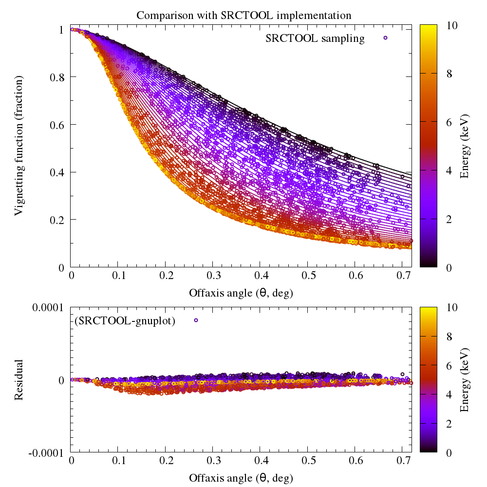
- The following plot shows that the SRCTOOL and gnuplot implementations give comparable results (within the numerical precision of this test)
