|
Size: 5668
Comment:
|
Size: 5766
Comment:
|
| Deletions are marked like this. | Additions are marked like this. |
| Line 23: | Line 23: |
| * See the gnuplot script used to do this: {{attachment:derive_analytic_vignetting_coeffs.plot}} |
Modelling the vignetting function of eROSITA
This is a holding page to gather together notes on producing an analytic vignetting model for eSASS tasks
Problem: The current method to represent the eROSITA vignetting function in the eSASS required interpolation from a tabulated grid of calibration measurements, this is computationally awkward, and can lead to discontinuities in the derived system response.
Desired improvement: Compute an analytic description of the vignetting function of each eROSITA telescope module, and save the parameters of this model into the CALDB.
Zeroth order model (TD)
Input data
- Start from the vignetting description file supplied with the current version of SIXTE
i.e. the file share/sixte/instruments/srg/erosita_vignetting_v2.1.fits supplied in the SIXTE instrument description package v1.4.0
- The file contains a list of vignetting values evaluated for broad energy bands and for many offaxis angles
- The vignetting is tabulated over 3 energy ranges: 0.0-2.5, 2.5-5.5 and 5.5-20 keV (in comparison eSASS uses energy ranges: 0.0-2.5, 2.5-5.5 and 5.5-10 keV)
- it is not clear what average or effective energy should be assumed for each energy band, for simplicity we assume 1.25keV, 4.0keV and 7.5keV.
- The vignetting is tabulated at 31 off-axis angles (from 0.0-30arcmin) for each energy band
- A single description is used for the vignetting functions of all eROSITA FMs/TMs
Derivation of model parameters
See the gnuplot script used to do this: derive_analytic_vignetting_coeffs.plot
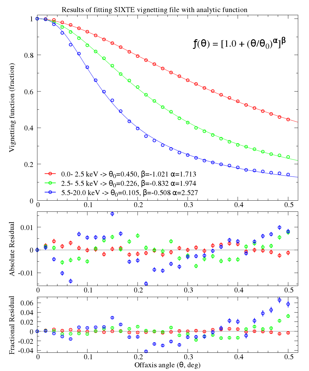
- For each energy value we fit a simple model to the vignetting as a function of off-axis angle (θ)
- For illustrative purposes we assume a uniform 1 sigma uncertainty of 1e-3 per data point
After some trial and error, a distribution of the form: vign(θ) = [1.0 + (θ/θ0)α]β was found to give a reasonable match to the tabulated values
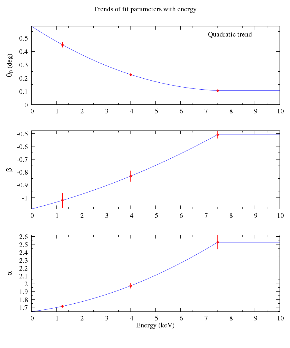
The values of the θ0,β,α parameters are then interpolated using a quadratic expression to allow evaluation of the expression at any energy
- This quadratic form does strange things at energies above the upper tabulated energy band and so the vignetting model is assumed to be constant in energy above 7.5keV
- future versions will be based on more energy bands (five or six?) than the three available here
   1 # See https://wiki.mpe.mpg.de/eRosita/EroCat/AnalyticVignetting
   2
   3
   4
   5 reset
   6 #set term qt
   7
   8 sixte_vignet_label = "SIXTE FM* (erosita_vignetting_v2.1.fits) "
   9 sixte_vignet = "/home/tdwelly/software/linux/share/sixte/instruments/srg/erosita_vignetting_v2.1.fits"
  10 sixte_vignet_nt=31
  11
  12 str_title_arith = "Arithmetic mean energy\nE_{mean}=(E_{lo}+E_{hi})/2"
  13 str_title_geom  = "Geometric mean energy\nE_{mean}=(E_{lo}.E_{hi})^{0.5}"
  14
  15 sixte_offaxis_unit_scale=60.0
  16 caldb_offaxis_unit_scale=1.0
  17
  18 str_fit_vars = 'avign_fit_vars.gnuplot'
  19
  20 print "Loading best fit variables from: ", str_fit_vars
  21 load str_fit_vars
  22
  23
  24 fit_vignetting = 0
  25 plot_fitted_model = 0
  26 plot_srctool_test = 1
  27
  28
  29 reset
  30
  31
  32 # fit the SIXTE vignetting with an analytic model - a psuedo-Moffat profile
  33 # https://en.wikipedia.org/wiki/Moffat_distribution
  34
  35
  36 vign0(oa,a,b,c) = ((1.0 + (oa/a)**c)**b)
  37 vign(oa) = vign0(oa,theta0,beta,alpha)
  38
  39 clip(eraw) = (eraw<emin?emin:(eraw>emax?emax:eraw))
  40
  41 # https://en.wikipedia.org/wiki/Lagrange_polynomial
  42 #l(x) = coeff_i[1]*((x-e[2])/(e[1]-e[2]))*((x-e[3])/(e[1]-e[3])) + coeff_i[2]*((x-e[1])/(e[2]-e[1]))*((x-e[3])/(e[2]-e[3])) + coeff_i[3]*((x-e[1])/(e[3]-e[1]))*((x-e[2])/(e[3]-e[2]))
  43 lagr(x,x1,x2,x3,y1,y2,y3) = y1*((x-x2)/(x1-x2))*((x-x3)/(x1-x3)) + y2*((x-x1)/(x2-x1))*((x-x3)/(x2-x3)) + y3*((x-x1)/(x3-x1))*((x-x2)/(x3-x2))
  44
  45 f_theta0(energy) = lagr(clip(energy),e[1],e[2],e[3],coeff_1[1],coeff_1[2],coeff_1[3])
  46 f_beta(energy)   = lagr(clip(energy),e[1],e[2],e[3],coeff_2[1],coeff_2[2],coeff_2[3])
  47 f_alpha(energy)  = lagr(clip(energy),e[1],e[2],e[3],coeff_3[1],coeff_3[2],coeff_3[3])
  48
  49 vign_gen(oa,energy) = vign0(oa,f_theta0(energy),f_beta(energy),f_alpha(energy))
  50
  51
  52 if ( fit_vignetting == 1 ) {
  53     emin = 0.0
  54     emax = 7.5
  55     ne = 3
  56     array e[ne] = [1.25, 4.0, 7.5]
  57     #array e[ne] = [1.25, 4.0, 6.5]
  58     array elo[ne] = [0.0, 2.5, 5.5]
  59     array ehi[ne] = [2.5, 5.5, 20.0]
  60
  61     array coeff_name[ne] = ["{/Symbol q}_0", "{/Symbol b}", "{/Symbol a}"]
  62     array coeff_1[ne] = [0.5, 0.2, 0.2]
  63     array coeff_2[ne] = [-1.0, -1.0, -1.0]
  64     array coeff_3[ne] = [2.0, 2.0, 2.0]
  65     array coeff_1_err[ne]
  66     array coeff_2_err[ne]
  67     array coeff_3_err[ne]
  68
  69
  70
  71     reset
  72     set fit prescale
  73     set fit errorvariables
  74     set fit logfile
  75     set fit quiet
  76
  77     infile_fmt =  "< gump %s ALL no | gawk -v ne=3 -v nt=%d -v ie=%d -v emid=%g '//{for(i=1;i<=ne;i++){elo[i]=$i;ehi[i]=$(i+ne)}; for(j=1;j<=nt;j++){t[j]=$(j+2*ne)};for(i=1;i<=ne;i++){print _;for(j=1;j<=nt;j++){v=$(2*ne+nt+1+(j-1)*ne+i); if(i==ie){err=1e-3;print emid,t[j],v, err}}}}'"
  78
  79     array infile_sixte[ne]
  80     infile_sixte[1] = sprintf(infile_fmt, sixte_vignet, sixte_vignet_nt, 1, e[1])
  81     infile_sixte[2] = sprintf(infile_fmt, sixte_vignet, sixte_vignet_nt, 2, e[2])
  82     infile_sixte[3] = sprintf(infile_fmt, sixte_vignet, sixte_vignet_nt, 3, e[3])
  83
  84     print infile_sixte[1]
  85     print infile_sixte[2]
  86     print infile_sixte[3]
  87
  88     do for [i=1:ne] {
  89
  90 	theta0 = coeff_1[i]
  91 	beta   = coeff_2[i]
  92 	alpha  = coeff_3[i]
  93 	fit [0:0.5] vign(x) infile_sixte[i] using 2 : 3 : 4 zerror via  theta0
  94 	fit [0:0.5] vign(x) infile_sixte[i] using 2 : 3 : 4 zerror via  theta0,beta
  95 	fit [0:0.5] vign(x) infile_sixte[i] using 2 : 3 : 4 zerror via  theta0,beta,alpha
  96
  97 	coeff_1[i] = theta0
  98 	coeff_2[i] = beta
  99 	coeff_3[i] = alpha
 100 	coeff_1_err[i] = theta0_err
 101 	coeff_2_err[i] = beta_err
 102 	coeff_3_err[i] = alpha_err
 103     }
 104
 105   save variables str_fit_vars
 106   print "Writing best fit variables to: ", str_fit_vars
 107 }
 108
 109
 110 if ( plot_fitted_model == 1 ) {
 111
 112     ##################################################
 113     # calculate the trends of the fit parameters with energy
 114     # - need quadratic trends to go through all points
 115     # f(x) = a*x**2 + b*x + c
 116
 117     do for [i=1:ne] {
 118         print sprintf("Energy=%8g keV: theta0=%8.5f +- %8.5f  beta=%8.5f +- %8.5f  alpha=%8.5f +- %8.5f", e[i], coeff_1[i], coeff_1_err[i], coeff_2[i], coeff_2_err[i], coeff_3[i], coeff_3_err[i])
 119     }
 120
 121     reset
 122     set term pngcairo size 1000,1200 font "Times,18"
 123     outfile = "fit_sixte_vignetting_with_moffat.png"
 124     print "Writing: ", outfile
 125     set out outfile
 126
 127     set cbrange [0:12]
 128     set palette maxcolors 12
 129     set xtics offset 0,0.6
 130     set key bottom left Left reverse samplen 2.0
 131     unset title
 132     set mxtics 5
 133     set mytics 2
 134     set format y "%5g"
 135     set ylabel offset 1.5,0
 136     set tmargin 0
 137     set bmargin 0
 138     set bar 0
 139     set xrange [0:0.52]
 140     set pointsize 1.5
 141
 142     set xlabel ""
 143     set multiplot title "Results of fitting SIXTE vignetting file with analytic function"
 144     set label 1 "{/Symbol \246}({/Symbol q}) = [1.0 + ({/Symbol q}/{/Symbol q}_0)^{/Symbol a}]^{/Symbol b} " at graph 0.6,0.85 font ",24"
 145     set ylabel "Vignetting function (fraction)"
 146     set size 1.0,0.5
 147     set origin 0.0,0.46
 148     set ytics auto
 149
 150     array str_label[ne]
 151     do for [i=1:ne] {
 152       str_label[i] = sprintf("%4.1f-%4.1f keV -> {/Symbol q}_0=%5.3f, {/Symbol b}=%6.3f {/Symbol a}=%5.3f",elo[i],ehi[i],coeff_1[i],coeff_2[i],coeff_3[i])
 153     }
 154     plot [][0:1.02]\
 155 	 infile_sixte[1] using 2 : 3 : 4 with yerrorbars pt 6 dt 1 lw 2 lc 1 t str_label[1] ,\
 156 	 infile_sixte[2] using 2 : 3 : 4 with yerrorbars pt 6 dt 1 lw 2 lc 2 t str_label[2] ,\
 157 	 infile_sixte[3] using 2 : 3 : 4 with yerrorbars pt 6 dt 1 lw 2 lc 3 t str_label[3] ,\
 158 	 vign0(x,coeff_1[1],coeff_2[1],coeff_3[1]) with lines lt 1 lc 1 not ,\
 159 	 vign0(x,coeff_1[2],coeff_2[2],coeff_3[2]) with lines lt 1 lc 2 not ,\
 160 	 vign0(x,coeff_1[3],coeff_2[3],coeff_3[3]) with lines lt 1 lc 3 not
 161
 162     unset label 1
 163     set size 1.0,0.2
 164     set origin 0.0,0.23
 165     set ytics -0.05,0.01,0.05
 166     set ylabel "Absolute Residual"
 167     plot [][]\
 168 	 (0.0) with lines lt -1 lw 0.5 not ,\
 169          infile_sixte[1] using 2 : ($3-vign0($2,coeff_1[1],coeff_2[1],coeff_3[1])) : ($4) with yerrorbars pt 6 lw 2 lc 1 t "",\
 170          infile_sixte[2] using 2 : ($3-vign0($2,coeff_1[2],coeff_2[2],coeff_3[2])) : ($4) with yerrorbars pt 6 lw 2 lc 2 t "",\
 171 	 infile_sixte[3] using 2 : ($3-vign0($2,coeff_1[3],coeff_2[3],coeff_3[3])) : ($4) with yerrorbars pt 6 lw 2 lc 3 t ""
 172
 173     set size 1.0,0.15
 174     set origin 0.0,0.05
 175     set ytics -0.1,0.02,0.1
 176     set ylabel "Fractional Residual"
 177     set xlabel "Offaxis angle ({/Symbol q}, deg)" offset 0,1.2
 178     plot [][]\
 179 	 (0.0) with lines lt -1 lw 0.5 not ,\
 180          infile_sixte[1] using 2 : (($3-vign0($2,coeff_1[1],coeff_2[1],coeff_3[1]))/$3) : ($4/$3) with yerrorbars pt 6 lw 2 lc 1 t "",\
 181          infile_sixte[2] using 2 : (($3-vign0($2,coeff_1[2],coeff_2[2],coeff_3[2]))/$3) : ($4/$3) with yerrorbars pt 6 lw 2 lc 2 t "",\
 182 	 infile_sixte[3] using 2 : (($3-vign0($2,coeff_1[3],coeff_2[3],coeff_3[3]))/$3) : ($4/$3) with yerrorbars pt 6 lw 2 lc 3 t ""
 183
 184     unset multiplot
 185     set out
 186     ##################################################
 187
 188     null = "< echo 0.0"
 189     reset
 190     set bar 0
 191     set term pngcairo size 1000,1200 font "Times,18"
 192     outfile = "fit_sixte_vignetting_with_moffat_params_vs_energy.png"
 193     print "Writing: ", outfile
 194     set out outfile
 195     set xlabel "" offset 0,1.0
 196
 197     set xtics 0,1,20 offset 0.0,0.3
 198     set ytics -3,0.1,3
 199     set mxtics 2
 200     set mytics 2
 201     set format y "%4g"
 202     set multiplot title "Trends of fit parameters with energy"
 203     set size 1.0,0.3
 204     set origin 0.0,0.65
 205     set ylabel "{/Symbol q}_0 (deg)" offset 1,0
 206     plot  [0:10][0:*] \
 207 	  f_theta0(x) with lines lc 3 t "Quadratic trend",\
 208 	  for [i=1:ne] null using (e[i]) : (coeff_1[i]) : (coeff_1_err[i])   with yerrorbars pt 6 lw 2 lc 1 t ""
 209
 210     set size 1.0,0.3
 211     set origin 0.0,0.35
 212     set ylabel "{/Symbol b}"
 213     plot  [0:10][] \
 214 	  f_beta(x) with lines lc 3 t "",\
 215 	  for [i=1:ne] null using (e[i]) : (coeff_2[i]) : (coeff_2_err[i])   with yerrorbars pt 6 lw 2 lc 1 t ""
 216
 217
 218     set size 1.0,0.3
 219     set origin 0.0,0.05
 220     set ylabel "{/Symbol a}"
 221     set xlabel "Energy (keV)"
 222     plot  [0:10][] \
 223 	  f_alpha(x) with lines lc 3 t "",\
 224 	  for [i=1:ne] null using (e[i]) : (coeff_3[i]) : (coeff_3_err[i])   with yerrorbars pt 6 lw 2 lc 1 t ""
 225
 226
 227     unset multiplot
 228     set out
 229     ##################################################
 230
 231     reset
 232     set term pngcairo size 1000,1000 font "Times,18"
 233     outfile = "fit_sixte_vignetting_analytic_model.png"
 234     print "Writing: ", outfile
 235     set out outfile
 236
 237     set cbrange [0:10]
 238     set xtics offset 0,0.6
 239     set key bottom left Left reverse samplen 2.0
 240     unset title
 241     set mxtics 5
 242     set mytics 2
 243     set format y "%5g"
 244     set ylabel offset 1.5,0
 245     set bar 0
 246     set xrange [0:0.52]
 247     set pointsize 1.5
 248
 249     set title "Analytic vignetting model derived from SIXTE vignetting file"
 250     set label 1 "{/Symbol \246}({/Symbol q},E) = [1.0 + [{/Symbol q}/{/Symbol q}_0(E)]^{/Symbol a(E)}]^{/Symbol b(E)}" at graph 0.4,0.95 font ",22"
 251     set ylabel "Vignetting function (fraction)"
 252     set ytics auto
 253     set cblabel "Energy (keV)"
 254     set xlabel "Offaxis angle ({/Symbol q}, deg)" offset 0,1.2
 255
 256     array str_label[ne]
 257     do for [i=1:ne] {
 258       str_label[i] = sprintf("Data %4.1f-%4.1f keV",elo[i],ehi[i])
 259     }
 260
 261     dummy = "< gawk 'BEGIN{for(oa=0.0;oa<=0.8;oa+=0.005){print oa};exit;}'"
 262     de = 0.5
 263     plot [][0:1.02]\
 264 	 for [energy_iter=0:50:1] dummy using ($1) : (vign_gen($1,energy_iter/5.0)) : (energy_iter/5.0) with lines lw 2 lt 1 lc palette not,\
 265 	 infile_sixte[1] using 2 : 3 : 4 : 1 with yerrorbars pt 6 dt 1 lw 2 lc palette t str_label[1] ,\
 266 	 infile_sixte[2] using 2 : 3 : 4 : 1 with yerrorbars pt 6 dt 1 lw 2 lc palette t str_label[2] ,\
 267 	 infile_sixte[3] using 2 : 3 : 4 : 1 with yerrorbars pt 6 dt 1 lw 2 lc palette t str_label[3]
 268
 269     set out
 270 }
 271 ######################################################################
 272 ######################################################################
 273 ######################################################################
 274 ######################################################################
 275
 276 if ( plot_srctool_test == 1 ) {
 277     # cd /home/tdwelly/working/SASS/tasks/srctool
 278     # source /home/tdwelly/erosita/scripts/sass-setup_local.csh eSASSdevel
 279     # make -f local_Makefile test > /home/tdwelly/erosita/eSASSvsSIXTE/srctool_avign_test_output.log
 280     infile_srctool= "< gawk '/AVIGNET_TEST / {print substr($0,32)}' /home/tdwelly/erosita/eSASSvsSIXTE/srctool_avign_test_output.log"
 281
 282     reset
 283     set term pngcairo size 1000,1000 font "Times,18"
 284     outfile = "test_srctool_avignet_module.png"
 285     print "Writing: ", outfile
 286     set out outfile
 287     set cblabel "Energy (keV)"
 288     set xlabel "Offaxis angle ({/Symbol q}, deg)" offset 0,0.8
 289     set xrange [0:0.72]
 290     set cbrange [0:10]
 291     set xtics offset 0,0.5
 292     set format y "%7g"
 293     set mxtics 5
 294     set mytics 2
 295
 296     dummy = "< gawk 'BEGIN{for(oa=0.0;oa<=0.8;oa+=0.005){print oa};exit;}'"
 297     de = 0.5
 298     set multiplot title "Comparison with SRCTOOL implementation"
 299
 300     set size 1.0,0.6
 301     set origin 0.0,0.38
 302     set key top right
 303     set ylabel "Vignetting function (fraction)" offset 1.5,0.0
 304     plot [][0:1.02]\
 305 	 for [energy_iter=0:50:1] dummy using ($1) : (vign_gen($1,energy_iter/5.0)) : (energy_iter/5.0) with lines lw 2 lt 1 lc palette not,\
 306 	 infile_srctool using 7 : 8 : 6 with points pt 6 dt 1 lw 2 lc palette t "SRCTOOL sampling"
 307
 308
 309     set key top left Right
 310     set size 1.0,0.4
 311     set origin 0.0,0.0
 312     set ylabel "Residual"
 313     set ytics -1e-4,1e-4,1e-4
 314     set mytics 10
 315     plot [][-1e-4:1e-4]\
 316 	infile_srctool using 7 : ($8-vign_gen($7,$6)) : 6 with points pt 6 dt 1 lw 2 lc palette t "(SRCTOOL-gnuplot)"
 317
 318
 319     unset multiplot
 320     set out
 321
 322 }
 323 ######################################################################
 324 ######################################################################
 325 ######################################################################
 326
 327
 328 exit
Figures demonstrating the fit


The parameters describing the model
Results of fits at each energy:
- functional form is:
vign(θ,θ0,β,α) = [1.0 + (θ/θ0)α]β
- where
- θ = off-axis angle in degrees
θ0 is a scaling parameter, also in degrees
- α, β are dimensionless exponents
- independent fits at each of [1.25, 4.0, 7.5] keV give:
Energy=    1.25 keV: theta0= 0.44966 +-  0.02004  beta=-1.02111 +-  0.05693  alpha= 1.71288 +-  0.01767
Energy=       4 keV: theta0= 0.22575 +-  0.00860  beta=-0.83151 +-  0.04289  alpha= 1.97408 +-  0.03523
Energy=     7.5 keV: theta0= 0.10547 +-  0.00350  beta=-0.50753 +-  0.03063  alpha= 2.52732 +-  0.09069
we can describe this as a matrix of coefficients [3 coeffs X Nenergies]
coeff[1,1],coeff[2,1],coeff[3,1] = [ 0.44966, -1.02111, 1.71288]
coeff[1,2],coeff[2,2],coeff[3,2] = [ 0.22575, -0.83151, 1.97408]
coeff[1,3],coeff[2,3],coeff[3,3] = [ 0.10547, -0.50753, 2.52732]
Since we only have three data points in energy, we use Lagrangian polynomial interpolation (https://en.wikipedia.org/wiki/Lagrange_polynomial)
- i.e if we have three points on the plane at (x1,y1), (x2,y2), (x3,y3), the quadratic equation that passes through all of them is given by:
lagr(x,x1,x2,x3,y1,y2,y3) = y1*((x-x2)/(x1-x2))*((x-x3)/(x1-x3)) + y2*((x-x1)/(x2-x1))*((x-x3)/(x2-x3)) + y3*((x-x1)/(x3-x1))*((x-x2)/(x3-x2))
- Therefore, energy dependent versions of theta0,beta,alpha are given by
f_theta0(energy) = lagr(clip(energy),e[1],e[2],e[3],coeff[1,1],coeff[1,2],coeff[1,3])
f_beta(energy)   = lagr(clip(energy),e[1],e[2],e[3],coeff[2,1],coeff[2,2],coeff[2,3])
f_alpha(energy)  = lagr(clip(energy),e[1],e[2],e[3],coeff[3,1],coeff[3,2],coeff[3,3])
- It is necessary to limit the extrapolation at high energies:
emin = 0.0
emax = 7.5
clip(eraw) = (eraw<emin?emin:(eraw>emax?emax:eraw))
- And so the general vignetting function is:
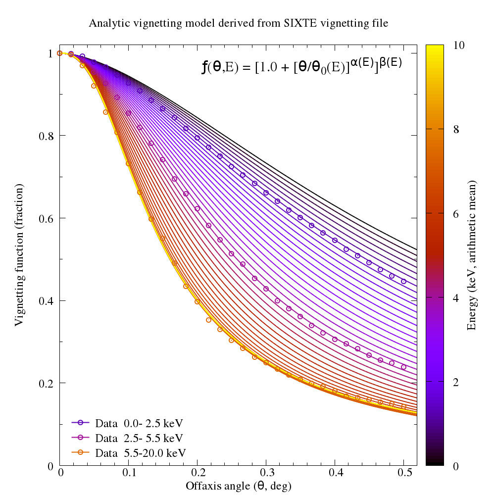
vign_gen(oa,energy) = vign(oa,f_theta0(energy),f_beta(energy),f_alpha(energy))
In the future we will have more energy intervals to consider and so a more sophisticated method will be needed to fit the trends of θ0,β,α as a function of energy
- The resultant analytic vignetting model is illustrated in the figure below:

Description of model in CALDB
- See script: "/home/erosita/sw/eSASSdevel/erosita/task/srctool/scripts/build_avign_caldb_files.csh"
- File format:
- One row per energy band
- Columns: Name, FITS format, Units
- ENERGY 1E [keV]
- COEFFS 3E [degree,-,-]
Using the analytic vignetting model in eSASS
- See module eSASS "/home/erosita/sw/eSASSdevel/erosita/task/srctool/srctool_generic_avign_mod.f90"