|
Size: 1252
Comment:
|
Size: 5199
Comment:
|
| Deletions are marked like this. | Additions are marked like this. |
| Line 1: | Line 1: |
| ## page was renamed from EroCalib/AnalyticVignetting | |
| Line 3: | Line 4: |
| ''This is a holding page to gather together notes on produsing an analytic vignetting model for eSASS tasks'' | ''This is a holding page to gather together notes on producing an analytic vignetting model for eSASS tasks'' |
| Line 10: | Line 11: |
| == First step == | = Zeroth order model (TD) = |
| Line 12: | Line 13: |
| * Start from the vignetting description file supplied with the current version of SIXTE (share/sixte/instruments/srg/erosita_vignetting_v2.1.fits) * this contains a list of vignetting values evaluated at 3 energies and 31 offaxis angles * For each energy value we fit a simple model as a function of off-axis angle * A pseudo-Moffat distribution is found to give a reasonable match to the data: vign(oa) = [1 + (oa/theta0)**alpha]**beta * The values of theta0,beta,alpha are then interpolated using a quadratic expression to allow evaluation of the expression at any energy |
== Input data == * Start from the vignetting description file supplied with the current version of SIXTE * i.e. the file share/sixte/instruments/srg/erosita_vignetting_v2.1.fits supplied in the [[http://www.sternwarte.uni-erlangen.de/research/sixte/downloads/sixte/instruments/instruments_srg-1.4.0.tar.gz|SIXTE instrument description package v1.4.0]] * The file contains a list of vignetting values evaluated for broad energy bands and for many offaxis angles * The vignetting is tabulated over 3 energy ranges: 0.0-2.5, 2.5-5.5 and 5.5-20 keV, eSASS uses energy ranges: 0.0-2.5, 2.5-5.5 and 5.5-10 keV * it is not clear what average or effective energy should be assumed for each energy band, for simplicity we assume 1.25keV, 4.5keV and 7.5keV. * The vignetting is tabulated at 31 off-axis angles (from 0.0-30arcmin) for each energy band * A single description is used for the vignetting functions of all eROSITA FMs/TMs |
| Line 18: | Line 22: |
| * The parameters describing the | == Derivation of model parameters == * For each energy value we fit a simple model to the vignetting as a function of off-axis angle (θ) * For illustrative purposes we assume a uniform 1 sigma uncertainty of 1e-3 per data point * After some trial and error, a distribution of the form: vign(θ) = [1.0 + (θ/θ,,0,,)^α^]^β^ was found to give a reasonable match to the tabulated values * The values of the θ,,0,,,β,α parameters are then interpolated using a quadratic expression to allow evaluation of the expression at any energy * This quadratic form does strange things at energies above the upper tabulated energy band and so the vignetting model is assumed to be constant in energy above 7.5keV * future versions will be based on more energy bands (five or six?) than the three available here === Figures demonstrating the fit === {{attachment:fit_sixte_vignetting_with_moffat.png|Vignetting model fitted to SIXTE file at defined energies|width=500}} {{attachment:fit_sixte_vignetting_with_moffat_params_vs_energy.png|Trends of vignetting model parameters with energy|width=500}} === The parameters describing the model === Results of fits at each energy: * functional form is: * vign(θ,θ,,0,,,β,α) = [1.0 + (θ/θ,,0,,)^α^]^β^ * where * θ = off-axis angle in degrees * θ,,0,, is a scaling parameter, also in degrees * α, β are dimensionless exponents * independent fits at each of [1.25, 4.0, 7.5] keV give: {{{ Energy= 1.25 keV: theta0= 0.44966 +- 0.02004 beta=-1.02111 +- 0.05693 alpha= 1.71288 +- 0.01767 Energy= 4 keV: theta0= 0.22575 +- 0.00860 beta=-0.83151 +- 0.04289 alpha= 1.97408 +- 0.03523 Energy= 7.5 keV: theta0= 0.10547 +- 0.00350 beta=-0.50753 +- 0.03063 alpha= 2.52732 +- 0.09069 }}} * we can describe this as a matrix of coefficients [3 coeffs X N,,energies,,] {{{ coeff[1,1],coeff[2,1],coeff[3,1] = [ 0.44966, -1.02111, 1.71288] coeff[1,2],coeff[2,2],coeff[3,2] = [ 0.22575, -0.83151, 1.97408] coeff[1,3],coeff[2,3],coeff[3,3] = [ 0.10547, -0.50753, 2.52732] }}} * It is necessary to limit the extrapolation at high energies: {{{ emin = 0.0 emax = 7.5 clip(eraw) = (eraw<emin?emin:(eraw>emax?emax:eraw)) }}} * We use lagrangian polynomial interpolation ([[https://en.wikipedia.org/wiki/Lagrange_polynomial]]) * i.e if we have three points on the plane at (x1,y1), (x2,y2), (x3,y3), the quadratic equation that passes through all of them is given by: {{{ lagr(x,x1,x2,x3,y1,y2,y3) = y1*((x-x2)/(x1-x2))*((x-x3)/(x1-x3)) + y2*((x-x1)/(x2-x1))*((x-x3)/(x2-x3)) + y3*((x-x1)/(x3-x1))*((x-x2)/(x3-x2)) }}} * Therefore, energy dependent versions of theta0,beta,alpha are given by {{{ f_theta0(energy) = lagr(clip(energy),e[1],e[2],e[3],coeff[1,1],coeff[1,2],coeff[1,3]) f_beta(energy) = lagr(clip(energy),e[1],e[2],e[3],coeff[2,1],coeff[2,2],coeff[2,3]) f_alpha(energy) = lagr(clip(energy),e[1],e[2],e[3],coeff[3,1],coeff[3,2],coeff[3,3]) }}} * And so the general vignetting function is: {{{ vign_gen(oa,energy) = vign(oa,f_theta0(energy),f_beta(energy),f_alpha(energy)) }}} {{attachment:fit_sixte_vignetting_analytic_model.png|Vignetting model at arbitrary energies|width=700}} == Description of model in CALDB == * See script: "/home/erosita/sw/eSASSdevel/erosita/task/srctool/scripts/build_avign_caldb_files.csh" == Using the analytic vignetting model in eSASS == * See module eSASS "/home/erosita/sw/eSASSdevel/erosita/task/srctool/srctool_generic_avign_mod.f90" |
Modelling the vignetting function of eROSITA
This is a holding page to gather together notes on producing an analytic vignetting model for eSASS tasks
Problem: The current method to represent the eROSITA vignetting function in the eSASS required interpolation from a tabulated grid of calibration measurements, this is computationally awkward, and can lead to discontinuities in the derived system response. Desired improvement: Compute an analytic description of the vignetting function of each eROSITA telescope module, and save the parameters of this model into the CALDB
Zeroth order model (TD)
Input data
- Start from the vignetting description file supplied with the current version of SIXTE
i.e. the file share/sixte/instruments/srg/erosita_vignetting_v2.1.fits supplied in the SIXTE instrument description package v1.4.0
- The file contains a list of vignetting values evaluated for broad energy bands and for many offaxis angles
- The vignetting is tabulated over 3 energy ranges: 0.0-2.5, 2.5-5.5 and 5.5-20 keV, eSASS uses energy ranges: 0.0-2.5, 2.5-5.5 and 5.5-10 keV
- it is not clear what average or effective energy should be assumed for each energy band, for simplicity we assume 1.25keV, 4.5keV and 7.5keV.
- The vignetting is tabulated at 31 off-axis angles (from 0.0-30arcmin) for each energy band
- A single description is used for the vignetting functions of all eROSITA FMs/TMs
Derivation of model parameters
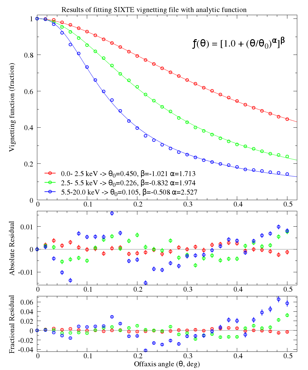
- For each energy value we fit a simple model to the vignetting as a function of off-axis angle (θ)
- For illustrative purposes we assume a uniform 1 sigma uncertainty of 1e-3 per data point
After some trial and error, a distribution of the form: vign(θ) = [1.0 + (θ/θ0)α]β was found to give a reasonable match to the tabulated values
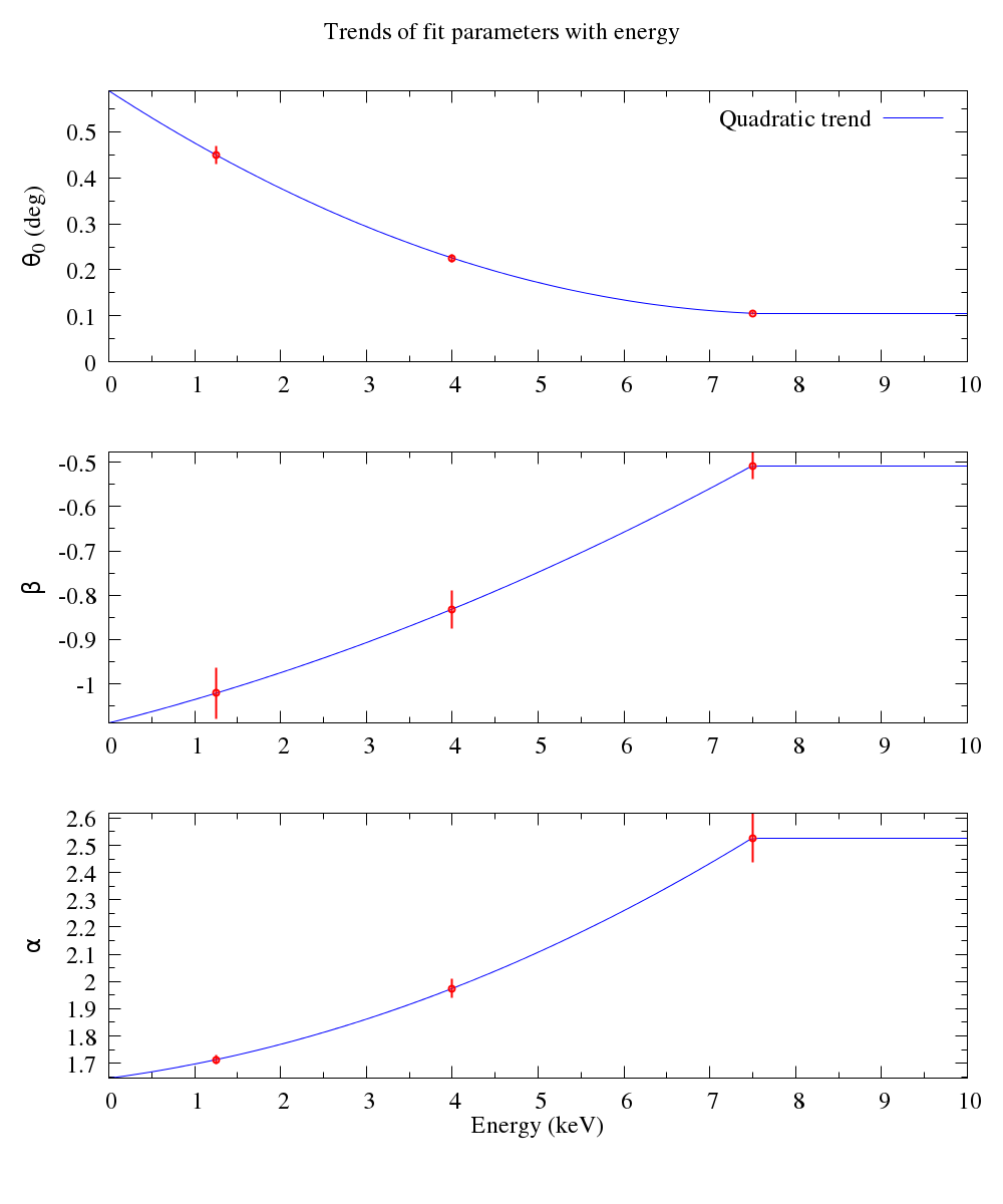
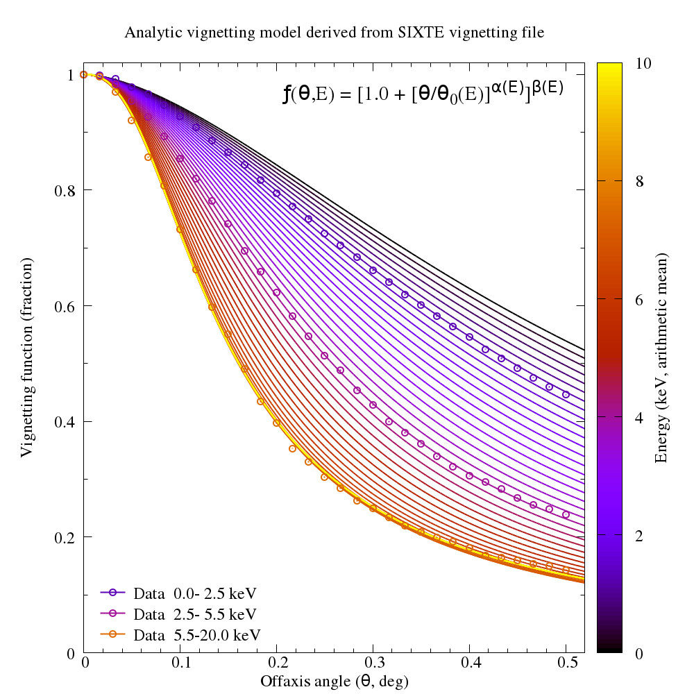
The values of the θ0,β,α parameters are then interpolated using a quadratic expression to allow evaluation of the expression at any energy
- This quadratic form does strange things at energies above the upper tabulated energy band and so the vignetting model is assumed to be constant in energy above 7.5keV
- future versions will be based on more energy bands (five or six?) than the three available here
Figures demonstrating the fit


The parameters describing the model
Results of fits at each energy:
- functional form is:
vign(θ,θ0,β,α) = [1.0 + (θ/θ0)α]β
- where
- θ = off-axis angle in degrees
θ0 is a scaling parameter, also in degrees
- α, β are dimensionless exponents
- independent fits at each of [1.25, 4.0, 7.5] keV give:
Energy=    1.25 keV: theta0= 0.44966 +-  0.02004  beta=-1.02111 +-  0.05693  alpha= 1.71288 +-  0.01767
Energy=       4 keV: theta0= 0.22575 +-  0.00860  beta=-0.83151 +-  0.04289  alpha= 1.97408 +-  0.03523
Energy=     7.5 keV: theta0= 0.10547 +-  0.00350  beta=-0.50753 +-  0.03063  alpha= 2.52732 +-  0.09069
we can describe this as a matrix of coefficients [3 coeffs X Nenergies]
coeff[1,1],coeff[2,1],coeff[3,1] = [ 0.44966, -1.02111, 1.71288]
coeff[1,2],coeff[2,2],coeff[3,2] = [ 0.22575, -0.83151, 1.97408]
coeff[1,3],coeff[2,3],coeff[3,3] = [ 0.10547, -0.50753, 2.52732]
- It is necessary to limit the extrapolation at high energies:
emin = 0.0
emax = 7.5
clip(eraw) = (eraw<emin?emin:(eraw>emax?emax:eraw))
We use lagrangian polynomial interpolation (https://en.wikipedia.org/wiki/Lagrange_polynomial)
- i.e if we have three points on the plane at (x1,y1), (x2,y2), (x3,y3), the quadratic equation that passes through all of them is given by:
lagr(x,x1,x2,x3,y1,y2,y3) = y1*((x-x2)/(x1-x2))*((x-x3)/(x1-x3)) + y2*((x-x1)/(x2-x1))*((x-x3)/(x2-x3)) + y3*((x-x1)/(x3-x1))*((x-x2)/(x3-x2))
- Therefore, energy dependent versions of theta0,beta,alpha are given by
f_theta0(energy) = lagr(clip(energy),e[1],e[2],e[3],coeff[1,1],coeff[1,2],coeff[1,3])
f_beta(energy)   = lagr(clip(energy),e[1],e[2],e[3],coeff[2,1],coeff[2,2],coeff[2,3])
f_alpha(energy)  = lagr(clip(energy),e[1],e[2],e[3],coeff[3,1],coeff[3,2],coeff[3,3])
- And so the general vignetting function is:
vign_gen(oa,energy) = vign(oa,f_theta0(energy),f_beta(energy),f_alpha(energy))

Description of model in CALDB
- See script: "/home/erosita/sw/eSASSdevel/erosita/task/srctool/scripts/build_avign_caldb_files.csh"
Using the analytic vignetting model in eSASS
- See module eSASS "/home/erosita/sw/eSASSdevel/erosita/task/srctool/srctool_generic_avign_mod.f90"